LaTeX writing as a constrained non-convex optimization problem

Martin Isaksson

13 min read June 6, 2020

Categories

• academia
• latex

Tags

• latex
• optimization

Table of contents

1. Introduction
   1. Contributions
2. Methods
   1. The LaTeX manuscript and a proxy quality metric
   2. Annotating the LaTeX source code
   3. Optimization problem
   4. Hyperparameter search
3. Results
   1. Track and visualize results
   2. Solutions found
4. Related work
5. Limitations, discussions and future work
6. Conclusions
7. Acknowledgment

The rejection rate for papers in good conferences is very high. To be accepted, a paper must not only be of a high scientific quality, but also at first impression perceived to be - or risk being thrown in the recycling bin. In this post we construct a system that automatically optimizes one proxy metric for perceived quality, removing one small frustrating step of scientific paper authorship and hopefully avoiding the bin.

Introduction

Scientific paper submission is a sort of empirical risk minimization problem where we want to minimize the risk that our paper will be rejected. We don’t have access to the true risk, but have to measure this empirical risk in some other way.

There are many factors that affect this risk - the most obvious being the quality of the content. However, with the increasing number of submissions the first impression of a reviewer is also increasingly important. In order for a reviewer to be able to assess the real quality of our paper, we must first avoid that the reviewer throws our paper into the recycling bin. A paper that successfully avoids the recycling bin should continue to convey a positive feeling so that the reviewer tries to find a reason to accept the paper rather than the opposite.

(Huang, 2018) trained a classifier to reject or accept a paper based solely on the visual appearance of a paper and found a few parameters that indicate good papers. One such interesting aspect is that we should fill all the available pages, which gives the impression of a more well-polished paper. In this post we will use this metric as a proxy for quality and minimize the empirical risk that our paper is rejected.

At submission time we find ourselves fighting the automated PDF checks of the publisher (see How to beat publisher PDF checks with L^aT_eX document unit testing) and we are changing figure sizes and other parameters, compiling and checking the output in order to fill the last page entirely and not have the content spill over to a new page. This process is frustrating, labor intensive, slow, and boring, not to mention error-prone.

The stuff from which nightmares are made - content spilling over to the fourth page.

A situation many of us recognize, regardless of where we are in our academic careers. With permission from "Piled Higher and Deeper" by Jorge Cham.

One large step towards a solution to this was proposed by (Acher et al., 2018) in which the authors annotate the L^aT_eX source with variability information. This information can be numerical values on figure sizes, or boolean values on options or whether to include certain paragraphs. In their work they formulate the learning problem as a constrained binary classification problem to classify into acceptable and non-acceptable configurations so that acceptable solutions can be presented to the user.

Here, we instead formulate this problem as a constrained optimization problem, where the constraints are defined by the automated PDF checks and the optimization is defined by proxy metrics such as amount of white space on the last page.

To find the optimal variable values we will use Ray Tune (Liaw et al., 2018). Ray Tune allows us to run parallel, distributed, L^aT_eX compilations and provides a large selection of search algorithms and schedulers.

Contributions

This work is inspired by three papers and develop these foundations in the following ways:

• We define and implement a proxy-metric for paper quality, based on findings from (Huang, 2018), that can be directly measured on a PDF-file. See Our L^aT_eX manuscript and a proxy quality metric.
• We show how a L^aT_eX document can be annotated using variability information following ideas from (Acher et al., 2018) but without using a preprocessor. See Annotating the L^aT_eX source code.
• We formulate a constrained non-convex objective function and proceed to solve it efficiently using Ray Tune (Liaw et al., 2018). See Optimization problem and Hyperparameter search.

Methods

The L^aT_eX manuscript and a proxy quality metric

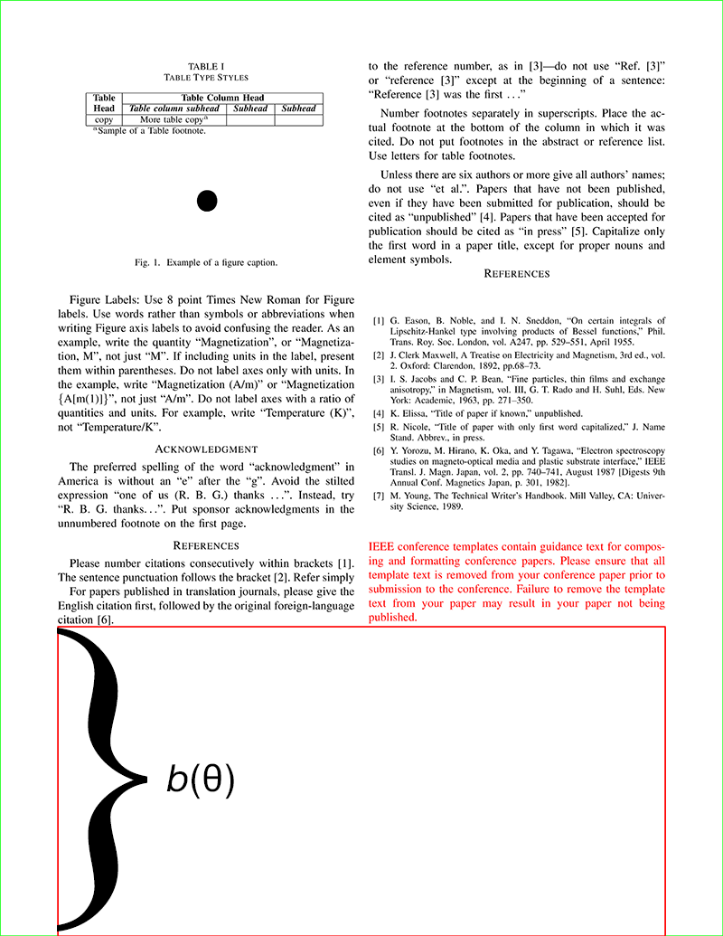
We again turn the example from the IEEE Manuscript Templates for Conference Proceedings to test these methods. The flushend package is used so that the last column is balanced. We also add another figure and vary each of the figure widths from zero width to one line widths - this will affect the amount of white space on the last page. A visualization of the last page white space can be seen in the figure below.

We use the example from the IEEE Manuscript Templates for Conference Proceedings to test these methods.

The cost we optimize is based on the bottom margin on the last page and depends on some input variables, such as figure widths.

def calculate_cost(self):

        pdf_document = fitz.open(self.pdffile)

        if pdf_document.pageCount > 3:
            return 10000

        page1 = pdf_document[-1]

        full_tree_y = IntervalTree()
        tree_y = IntervalTree()

        blks = page1.getTextBlocks()  # Read text blocks of input page

        # Calculate CropBox & displacement
        disp = fitz.Rect(page1.CropBoxPosition, page1.CropBoxPosition)

        croprect = page1.rect + disp
        full_tree_y.add(Interval(croprect[1], croprect[3]))

        for b in blks:  # loop through the blocks
            r = fitz.Rect(b[:4])  # block rectangle

            # add dislacement of original /CropBox
            r += disp
            _, y0, _, y1 = r

            tree_y.add(Interval(y0, y1))

        tree_y.merge_overlaps()

        for i in tree_y:
            full_tree_y.add(i)

        full_tree_y.split_overlaps()

        # For top and bottom margins, we only know they are the first and
        # last elements in the list
        full_tree_y_list = list(sorted(full_tree_y))
        _, bottom_margin = \
            map(
                get_interval_width,
                full_tree_y_list[::len(full_tree_y_list) - 1]
            )

        return bottom_margin

To calculate our metric it will be required to find the dimensions of each page and each bounding box within the last page (Isaksson, 2020).

The basic algorithm is as follows: We loop over each bounding box within the last page. For every bounding box we add an interval to an interval tree for the dimensions in the y-direction. We can the use this to find the difference between the page dimensions and the extent of the bounding boxes on the page. For this we will use the Python package intervaltree (Leib Halbert & Tretyakov, 2018).

The implementation is discussed more in How to beat publisher PDF checks with L^aT_eX document unit testing.

Annotating the L^aT_eX source code

For this example, we will vary the width of two figures, in terms of \linewidth. The value of each variable is sampled from \(\mathcal{U}\left(0,1\right)\).

Variable	Variable name	Type	Space	Unit
The width of Figure 1.	figonewidth	float	\(\mathcal{U}\left(0,1\right)\)	ratio of \linewidth
The width of Figure 2.	figonewidth	float	\(\mathcal{U}\left(0,1\right)\)	ratio of \linewidth

To make things easy for us, we write variable definitions to a macros.tex file and input this file in our L^aT_eX document preamble. The file contains for example the definitions for two figure width.

\def\figonewidth{0.602276759098264}
\def\figtwowidth{0.5600851582135735}

These variables are then used in the document to set each figure width individually. As an example, here is the first figure:

\begin{figure}[htbp]
\centering
\includegraphics[width=\figonewidth\linewidth]{fig1.png}
\caption{Example of a figure caption.}
\label{fig1}
\end{figure}

In this way we can avoid using a pre-processor, and we can use only L^aT_eX code in the document itself. Note that we do not specify the domain of these variables in the L^aT_eX-code, but define this in the Python-code instead, see Defining the experiment. In our work, these variables can be of any data type that is supported in L^aT_eX and Python.

Optimization problem

Our objective function is based on the last page bottom margin \(b(\boldsymbol{\theta})\) that is a function of our variables \(\boldsymbol{\theta} = \left[\theta_0, \ldots, \theta_n\right]\). We add a L2-regularization term on \(1-\theta_k\) for each variable \(\theta_k \in \boldsymbol{\theta}\) since we want to favor solutions with larger \(\theta_k\), solutions that have similar \(\theta_k\) and to make the math look more impressive. We negate the objective function and maximize it. If requirements set out in How to beat publisher PDF checks with L^aT_eX document unit testing are not met, we add a penalty to \(l(\boldsymbol{\theta})\).

The optimal variables \(\boldsymbol{\theta}*\) are then

\[\boldsymbol{\theta}^* = \underset{\boldsymbol{\theta}}{\operatorname{argmax}} -1 \left(l(\boldsymbol{\theta}) + \lambda \sum_{k=1}^n \left(1-\theta_k\right)^2\right)\]

where

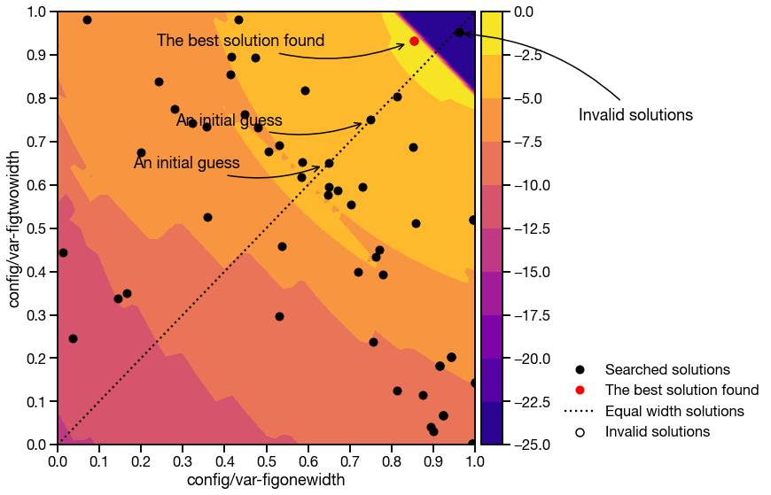
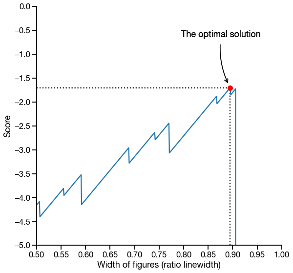
\[l(\boldsymbol{\theta}) = \begin{cases} b(\boldsymbol{\theta}) & \text{if constraints are met.}\\ 10000 & \text{otherwise.} \end{cases}\]

As we can see in the figures below, the objective function \(l(\bf{\theta})\) is non-convex and the added L2-regularization gives us solutions that tend to have larger figure widths, which is what we want.

Our objective function depends on the two figure widths figonewidth and figonewidth.

The objective function with L2-regularization is more well-behaving, but note the lack of symmetry around the diagonal.

Note that we cannot tune the hyper-parameter \(\lambda\), so we set it to \(2\pi\), because that’s the most beautiful number known to man.

Hyperparameter search

Defining the tasks

We will use Ray Tune (Liaw et al., 2018) for searching this parameter space (the parameters we are defining here are of course not hyper-parameters). We begin with an exhaustive grid-search over the entire search space which is here \(v \in [0, 1]\, \forall \theta_k \in \boldsymbol{\theta}\). Since we have two figures each with a variable width we have \(\vert\boldsymbol{\theta}\vert = 2\). Performing a grid-search over each of the variables divided into 51 possible values gives us 2601 paper variants to compile. Each of the paper compilations consists of five steps;

1. Copy the L^aT_eX code to a temporary directory.
2. Sample variables and write to file macros.tex,
3. Clean document directory using latexmk and
4. Compile document with latexmk.
5. Measure quality proxy-metrics on PDF file.

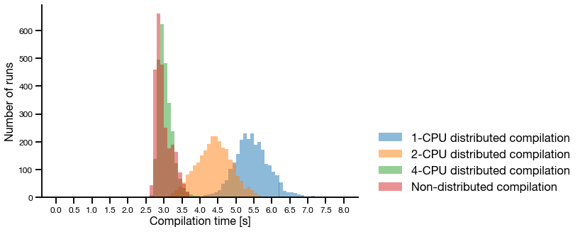
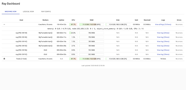
The average execution time for each task is 5.46 seconds, and we can run 8 of these in parallel. This means that an experiment takes roughly 30 minutes on my laptop. With Ray Tune we also have the option to run this using a much larger set of machines if needed. Compilation using more than one CPU per worker is shorter, but since we can run fewer in parallel the total execution time is longer.

Document compilation (really Ray worker execution) time PDF, because measuring things makes it feel more like science.

Search algorithm

However, running an exhaustive grid search is not needed as we can use one of the search algorithms provided by Ray Tune instead. Specifically we will use a Asynchronous HyperBand scheduler with a HyperOpt search algorithm. HyperOpt (Bergstra et al., 2013) is a Python library for optimization over awkward search spaces. In our use-case we have real-valued, discrete and conditional variables so this library works for us, but we will not evaluate its performance on our objective function and can therefore not claim that it is the best search algorithm for this particular problem.

Defining the experiment

We define our experiment directly in the code, for simplicity. First we will define our search space. Here we sample each variable from \(\mathcal{U}(0,1)\).

space = {
    'var-figonewidth': hp.uniform('var-figonewidth', 0, 1),
    'var-figtwowidth': hp.uniform('var-figtwowidth', 0, 1),
}

We can then optionally give a few starting guesses. We will give to guesses that both lie on the diagonal where both figure widths are equal.

current_best_params = [
    {'var-figonewidth': .75, 'var-figtwowidth': .75},
    {'var-figonewidth': .65, 'var-figtwowidth': .65}
]

Lastly we will define our Ray Tune experiment and run it.

algo = HyperOptSearch(space, metric="score", mode="max",
                      points_to_evaluate=current_best_params)

scheduler = AsyncHyperBandScheduler(metric="score", mode="max")

tune.run(
    MyTrainable, name=config["name"],
    scheduler=scheduler, search_alg=algo,
    config=conf, verbose=1,
    resources_per_trial=config["resources"],
    num_samples=num_samples_per_axis,
    reuse_actors=True,
    loggers=DEFAULT_LOGGERS + (MLFLowLogger, ))

See the complete source code in the repository.

Results

Track and visualize results

We can visualize the results of the hyper-parameter search using Tensorboard (Abadi et al., 2015) in a Docker (Merkel, 2014) container using the following command:

docker run -v [RAY_RESULTS_PATH]:/tf_logs -p 6006:6006 tensorflow/tensorflow:2.1.1 tensorboard --bind_all --logdir /tf_logs

Visualizing L^aT_eX compilation metrics via Ray Tune using Tensorboard in Docker ticks all the nerd-boxes.

Ray Tune integrates well with MLFlow. Here we use the Parallel Coordinates Plot to visualize invalid solutions.

The Ray dashboard provides a minimal dashboard to monitor the workers.

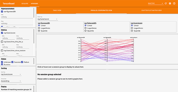
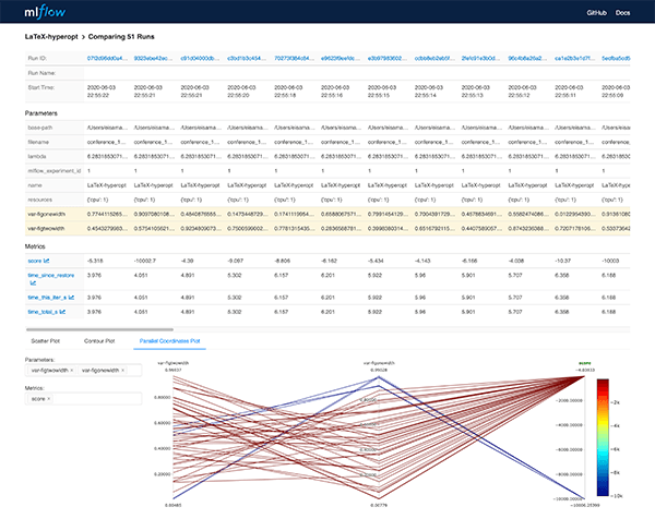
MLFlow (Databricks, 2020) is a Python package that can be used to for example track experiments and models. Here we use it to visualize the hyper-parameters and the corresponding objective function score. The MLFLow UI can be started simply with mlflow ui.

Solutions found

The objective function with L2-regularization visualized with solutions searched by HyperOpt.

Objective function score as a function of figure widths when both figures are set to equal width. Note that the optimal solution is not the maximum figure width that still satisfies the constraints.

For the specific objective function illustrated here, we could potentially use a variant of gradient descent. However, as we add more variables, the search space becomes more complicated.

Using Ray Tune has a major advantage in that it is easy to parallelize our document compilation on a large set of workers and the API makes changing scheduler and search algorithm a breeze.

Related work

In the inspiring “VaryL^aT_eX: Learning Paper Variants That Meet Constraints” paper (Acher et al., 2018) the authors annotate L^aT_eX source with variability information and construct a binary classification problem where the aim is to classify a configuration as fulfilling the constraints or not. The classifier can be used to present a set of configurations to the user that then can pick an aesthetically pleasing configuration out of the presented set. This is a much more complete solution that the one presented in this post. A potentially interesting addition to their work is to annotate the configurations with a score, that can be used to sort a potentially large set of valid configurations. See their Github repository.

(Huang, 2018) constructs a binary classification tasks to predict if a paper is good or bad, based on the Paper Gestalt of a paper, i.e. only the visual representation of the paper. The paper goes on to discuss how to improve the Paper Gestalt, for example adding a teaser figure, a figure on the last page and filling the complete last page. The latter can be numerically estimated, which is what we based this blog post on.

Limitations, discussions and future work

The experiments in this blog post aim to produce a single paper that fulfills all publisher constrains and requirements. This single paper is optimized in terms of last page white space, which disregards pretty much everything that makes a paper great and should therefore be used with caution.

There are other metrics that we can use for optimization, for example the number of words, data density (Tufte, 1986). We can add more variability by considering figure placement, microtype options (Schlicht, 2019), and more.

The optimization can be added as a stage in a L^aT_eX pipeline as outlined in How to annoy your co-authors: a Gitlab CI pipeline for L^aT_eX

In this post we viewed the parameters as hyper-parameter and used Ray Tune, which is made for tuning hyper-parameters . The parameters we used are in fact not hyper-parameters, and other frameworks and solvers could have been used. However, we find that two aspects of Ray Tune makes it a good candidate for this problem; it’s is simple to use and it can parallelize these tasks efficiently.

Conclusions

While the last page white space is obviously a bad proxy for paper quality, we have shown that we can remove a part of paper writing that is labor intensive, slow, boring, and error-prone. We combined three pieces of work that I find ingenious in their own rights to make a complicated machine to optimize a parameter that maybe doesn’t matter all that much - but, hey, it was fun!

Acknowledgment

This post has been in the making for a very long time, but it was a comment on How to beat publisher PDF checks with L^aT_eX document unit testing by @mathieu_acher that finally made me sit down and make this happen. Thank you!

References

1. Huang, J.-B. (2018). Deep Paper Gestalt. CoRR, abs/1812.0. http://arxiv.org/abs/1812.08775
2. Acher, M., Temple, P., Jezequel, J.-marc, Galindo, J. Á., Acher, M., Temple, P., Jezequel, J.-marc, Ángel, J., Duarte, G., Martinez, J., Temple, P., & Jézéquel, J.-marc. (2018). VaryLaTeX : Learning Paper Variants That Meet Constraints. VaMoS 2018 - 12th International Workshop on Variability Modelling of Software-Intensive Systems. https://doi.org/10.1145/3168365.3168372
3. Liaw, R., Liang, E., Nishihara, R., Moritz, P., Gonzalez, J. E., & Stoica, I. (2018). Tune: A Research Platform for Distributed Model Selection and Training. ArXiv Preprint ArXiv:1807.05118.
4. Isaksson, M. (2020). Martin’s blog - How to beat publisher PDF checks with LaTeX document unit testing.
5. Leib Halbert, C., & Tretyakov, K. (2018). intervaltree. https://pypi.org/project/intervaltree/
6. Bergstra, J., Yamins, D., & Cox, D. D. (2013). Making a Science of Model Search: Hyperparameter Optimization in Hundreds of Dimensions for Vision Architectures. Proceedings of the 30th International Conference on Machine Learning, ICML 2013, Atlanta, GA, USA, 16-21 June 2013, 28, 115–123. http://proceedings.mlr.press/v28/bergstra13.html
7. Abadi, M., Agarwal, A., Barham, P., Brevdo, E., Chen, Z., Citro, C., Corrado, G. S., Davis, A., Dean, J., Devin, M., Ghemawat, S., Goodfellow, I., Harp, A., Irving, G., Isard, M., Jia, Y., Rafal Jozefowicz, Kaiser, L., Kudlur, M., … Zheng, X. (2015). TensorFlow: Large-Scale Machine Learning on Heterogeneous Systems. https://www.tensorflow.org/
8. Merkel, D. (2014). Docker: Lightweight Linux Containers for Consistent Development and Deployment. Linux J., 2014(239). http://dl.acm.org/citation.cfm?id=2600239.2600241
9. Databricks. (2020). MLFlow. https://www.mlflow.org/
10. Tufte, E. R. (1986). The Visual Display of Quantitative Information. Graphics Press. https://www.edwardtufte.com/tufte/books_vdqi
11. Schlicht, R. (2019). Microtype. 1–249. https://ctan.org/pkg/microtype

Suggested citation

If you would like to cite this work, here is a suggested citation in BibTeX format.

@misc{isaksson_2020,
  author="Isaksson, Martin",
  title={{Martin's blog --- LaTeX writing as a constrained non-convex optimization problem}},
  year=2020,
  url=https://blog.martisak.se/2020/06/06/latex-optimizer/,
  note = "[Online; accessed 2024-04-07]"
}

Share Tweet LinkedIn Reddit

Revisions