

Tables in scientific papers often look less than professional, and sometimes
this can even get in the way of understanding the message. Unless the message is
“Massive tables indicate scientific rigour”. In this blog post we will use
pandas to automate making publication ready LaTeX tables that look great.
Updated July 2026
Updated for full reproducibility. table.py now pins its exact dependencies (pandas==3.0.3, seaborn==0.13.2, jinja2==3.1.6) via inline PEP 723 script metadata and runs with uv run. The LaTeX compile step runs inside a digest-pinned texlive/texlive Docker image, so it’s the same TeX Live install regardless of what’s on your machine or when you run it. make drives the whole pipeline end to end.
Introduction
Tufte argues that we should strive to have a high data to ink-ratio (Tufte, 1986) which means that we should strive to remove redundant graphical element that do not contribute to conveying our message. This applies to tables as well.
For typesetting tables in my scientific papers I use LaTeX with the booktabs
(Fear & Els, 2020) package, one of my top 10 LaTeX packages. It is either my absolute favorite, or
maybe a runner-up. Using booktabs goes a long way towards making beautiful
tables with a high data to ink-ratio, but it’s a manual process.
In this blog post we will explore automating tables using pandas (pandas development team, 2020; Wes McKinney, 2010 ) and booktabs for removing some
unwanted ink from our tables. Building a pipeline for generating and including
the tables into our LaTeX papers has the huge benefit of being reproducible.
Because typesetting tables manually belongs in the 1980s.
Not saying you should group the data in this particular way, this post is just showing you could. In our post on adding sparklines we look into adding sparklines to our tables, and honestly you should read Tufte’s (Tufte, 1986) books before making tables anyways.
Using pandas to make a table
The first thing we need to do is to make a table from a dataset. We’ll look at
the Iris dataset (Fisher, 1936) from the seaborn (Waskom, 2021) Python library.
Fisher’s 1936 paper printed this data as a hand-typeset “Table I” — fifty rows for each of three species. Here’s how the first few rows of Iris setosa looked in print:
| Sepal length | Sepal width | Petal length | Petal width |
|---|---|---|---|
| 5.1 | 3.5 | 1.4 | 0.2 |
| 4.9 | 3.0 | 1.4 | 0.2 |
| 4.7 | 3.2 | 1.3 | 0.2 |
| 4.6 | 3.1 | 1.5 | 0.2 |
| 5.0 | 3.6 | 1.4 | 0.2 |
| 5.4 | 3.9 | 1.7 | 0.4 |
| 4.6 | 3.4 | 1.4 | 0.3 |
| 5.0 | 3.4 | 1.5 | 0.2 |
| 4.4 | 2.9 | 1.4 | 0.2 |
| 4.9 | 3.1 | 1.5 | 0.1 |
These are the same measurements seaborn.load_dataset('iris') still ships
today — the dataset every pandas tutorial reaches for is, quite literally,
Fisher’s.
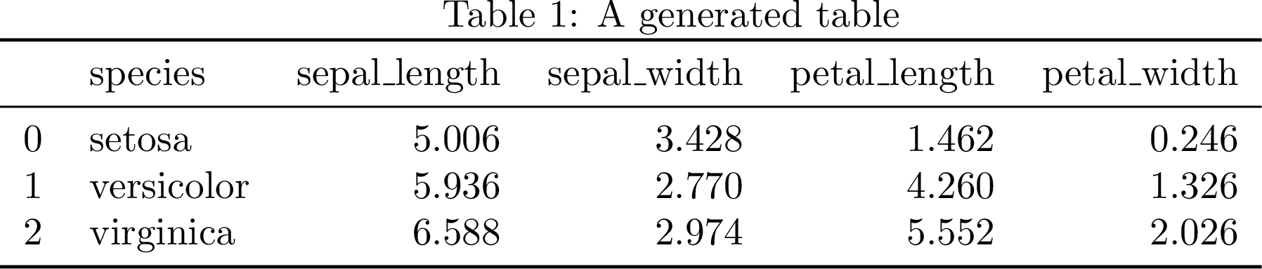
We could simply use the pandas function
to_latex()
to save a file containing the table in LaTeX format. pandas requires
booktabs, but we can make this table even more beautiful with some simple tweaks.
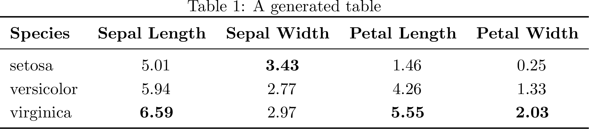
We want a few things from this table: mean and standard deviation per
measurement, with Length and Width as the two column groups (each under a
\cmidrule) and Sepal/Petal down the rows, one species block per pair of
rows separated by a dashed rule, and the largest mean per dimension highlighted
in bold.
pandas.DataFrame.agg(["mean", "std"]) gives a 2-level column index
(sepal_length, mean), (sepal_length, std), and so on. Each of those
column names carries two facts at once — the organ (Sepal/Petal) and the
dimension (Length/Width) — so we first split them on _ into a 3-level
(Organ, Dimension, Statistic) column index. That split comes straight
from the data’s own column names rather than being typed out by hand, so it
stays correct even if the underlying dataset changes.
The layout choice matters here. The comparison worth inviting is sepal-vs-petal
within a dimension. Here we compare a sepal length against a petal length,
same units, same axis. Those belong in the same column, one row apart.
Length-vs-width is a comparison of orthogonal dimensions we’d rather not
invite, so we keep it split across two column groups. To get that, we stack()
the Organ level down into the row index: rows become (Species, Organ),
columns become just (Dimension, Statistic). This also collapses the header
from three rows to two.
From there we use DataFrame.style rather than the plain to_latex()
call, since we need per-cell formatting to_latex() alone can’t express.
Styler.highlight_max() bolds the largest mean in each dimension column — no
manual string patching required, unlike the version of this post from
before pandas’ Styler-based LaTeX export existed. Styler.format_index()
bolds the Length/Width group labels and swaps the plain mean/std
labels for \mu/\sigma; those get wrapped in {} so siunitx’s S
columns don’t try to parse them as numbers (the same trick as the
Price ($) header in the booktabs example). We still use siunitx (Wright, 2009) — see Top LaTeX commands and macros for more examples — but its job is now
just column alignment (S[table-format=1.2]), since Styler.format(precision=2)
does the actual rounding on the Python side before the value ever reaches LaTeX.
Two gaps are left to patch in the rendered LaTeX. First, Styler.to_latex()
prints the row-index names (Species, Organ) as their own header row; we
fold those two labels into the empty leading cells of the \mu/\sigma row and
drop the redundant line, bolding them to match the Length/Width headers, so
the header is exactly the two rows we want. Second, it renders the grouped
\multicolumn header without a \cmidrule underneath, so we add one with a
small generic helper, cmidrules(), that walks the same MultiIndex the
columns are built from and emits one rule per contiguous group — derived from
the actual column structure rather than hardcoded. Finally, we separate each
species block with a dashed \hdashline (from the arydshln package), so the
two-row-per-species grouping reads at a glance.
1
2
3
4
5
6
7
8
9
10
11
12
13
14
15
16
17
18
19
20
21
22
23
24
25
26
27
28
29
30
31
32
33
34
35
36
37
38
39
40
41
42
43
44
45
46
47
48
49
50
51
52
53
54
55
56
57
58
59
60
61
62
63
64
65
66
67
68
69
70
71
72
73
74
75
76
77
78
79
80
81
82
83
84
85
86
87
88
89
90
91
92
93
94
95
96
97
98
99
100
101
102
103
104
105
106
107
108
109
110
111
112
113
114
115
116
117
118
119
120
121
122
123
124
125
126
127
128
129
130
131
132
133
134
135
136
137
138
139
140
141
142
143
144
145
146
147
148
149
150
151
152
153
154
155
156
157
158
159
160
161
# /// script
# requires-python = ">=3.10"
# dependencies = [
#     "pandas==3.0.3",
#     "seaborn==0.13.2",
#     "jinja2==3.1.6",
# ]
# ///
import os

import pandas as pd
import seaborn as sns


def cmidrules(columns, level, start_col=1):
    """Emit one `\\cmidrule` per contiguous run of equal, non-empty labels
    at the given MultiIndex level. Generic over the actual column
    structure: add, remove, or rename groups and the rules follow.
    """
    rules = []
    run_start = None
    prev_key = None
    cols = list(columns)
    for i, col in enumerate(cols):
        pos = start_col + i
        key = col[: level + 1]
        label = col[level]
        same_run = key == prev_key and label != ""
        if not same_run:
            if run_start is not None and prev_key[-1] != "":
                span = str(run_start) + "-" + str(pos - 1)
                rules.append(r"\cmidrule(lr){" + span + "}")
            run_start = pos if label != "" else None
        prev_key = key
    if run_start is not None and prev_key[-1] != "":
        span = str(run_start) + "-" + str(start_col + len(cols) - 1)
        rules.append(r"\cmidrule(lr){" + span + "}")
    return "".join(rules)


if __name__ == "__main__":

    # Load data and calculate mean and std of each column, per species.
    agg = (sns.load_dataset('iris')
           .groupby("species")
           .agg(["mean", "std"])
           )

    # The (sepal_length, mean) columns pandas gives us carry two facts in
    # one name: the organ (Sepal/Petal) and the dimension (Length/Width).
    # Split them into a 3-level (Organ, Dimension, Statistic) column index,
    # straight from the column names so this stays correct if the data
    # changes.
    agg.columns = pd.MultiIndex.from_tuples(
        [(c[0].split("_")[0].title(),
          c[0].split("_")[1].title(),
          c[1]) for c in agg.columns],
        names=["Organ", "Dimension", "Statistic"],
    )

    # The comparison that matters is sepal-vs-petal *within* a dimension
    # (a sepal length against a petal length -- same units, same axis),
    # so those belong in the same column, one row apart. Length-vs-width
    # is a comparison of orthogonal dimensions we'd rather not invite, so
    # it's split across two column groups instead. Move Organ down into
    # the row index to make that layout: rows become (Species, Organ),
    # columns become (Dimension, Statistic).
    tbl = agg.stack(level="Organ", future_stack=True)

    # Fix the row order (stack sorts): Setosa/Versicolor/Virginica, each
    # with Sepal above Petal.
    species = ["setosa", "versicolor", "virginica"]
    tbl = tbl.reindex(
        pd.MultiIndex.from_product(
            [species, ["Sepal", "Petal"]], names=["Species", "Organ"]),
    )
    tbl.index = tbl.index.set_levels(
        [s.title() for s in species], level="Species")

    # Drop the column-axis names: with Organ moved into the rows, the
    # remaining levels are just Dimension/Statistic, and we don't want
    # those words printed as a header row -- the two-row header should be
    # Length/Width over mu/sigma, nothing more.
    tbl.columns.names = [None, None]

    mean_cols = [c for c in tbl.columns if c[1] == "mean"]

    styler = (
        tbl.style
        .format(precision=2)
        # Bold the largest mean in each dimension column -- Styler-native,
        # so no manual string patching of the rendered LaTeX is needed.
        .highlight_max(subset=mean_cols, props="bfseries:--rwrap;")
        # Bold the top-level (Length/Width) group labels.
        .format_index(
            lambda v: r"\textbf{" + v + "}" if v else v, axis=1, level=0)
        # mu/sigma read better than "mean"/"std" in a compact table; the
        # braces protect them from siunitx's S-column number parsing.
        .format_index(
            lambda v: r"{$\mu$}" if v == "mean" else
            r"{$\sigma$}" if v == "std" else v,
            axis=1, level=1)
    )

    column_format = "ll" + "S[table-format=1.2]" * len(tbl.columns)
    table = styler.to_latex(
        column_format=column_format,
        hrules=True,
        sparse_index=True,
        sparse_columns=True,
        multicol_align="c",
    )

    lines = table.splitlines()

    # pandas prints the row-index names (Species, Organ) as their own
    # header row, below the mu/sigma row and left of empty data cells.
    # Fold those two labels into the empty leading cells of the mu/sigma
    # row and drop the now-redundant names row, so the header is exactly
    # two rows: Length/Width, then Species | Organ | mu sigma mu sigma.
    n_index = tbl.index.nlevels
    index_names = list(tbl.index.names)
    for i, line in enumerate(lines):
        cells = line.rstrip(r"\ ").split("&")
        if [c.strip() for c in cells[:n_index]] == index_names:
            # Bold the row-axis header words (Species, Organ) to match the
            # bold Length/Width column headers; data values stay roman.
            name_cells = [r" \textbf{" + n + "} " for n in index_names]
            stat_cells = lines[i - 1].rstrip(r"\ ").split("&")
            merged = name_cells + stat_cells[n_index:]
            lines[i - 1] = "&".join(merged).rstrip() + r" \\"
            del lines[i]
            break

    # `to_latex` doesn't add a `\cmidrule` under the grouped Length/Width
    # header, so add one, computed from the same MultiIndex the columns
    # are built from. The two index columns (Species, Organ) push the
    # data columns to start at column 3.
    toprule_i = lines.index(r"\toprule")
    lines.insert(toprule_i + 2, cmidrules(tbl.columns, 0, start_col=3))

    # Separate each species block with a dashed rule (arydshln). Body rows
    # sit between `\midrule` and `\bottomrule`; there are two organ rows
    # per species, so a `\hdashline` goes after every second body row
    # except the last.
    midrule_i = lines.index(r"\midrule")
    bottomrule_i = lines.index(r"\bottomrule")
    body = lines[midrule_i + 1:bottomrule_i]
    rebuilt = []
    for i, row in enumerate(body):
        rebuilt.append(row)
        if i % 2 == 1 and i != len(body) - 1:
            rebuilt.append(r"\hdashline")
    lines = lines[:midrule_i + 1] + rebuilt + lines[bottomrule_i:]
    table = "\n".join(lines)

    # Write to file
    with open(
        os.path.splitext(
            os.path.basename(__file__))[0] + ".tbl", "w") as f:
        f.write(table)
At the end we are using the pandas function to_latex() to generate the LaTeX code and write the result to a file containing the tabular environment. The script pins its own exact dependencies (pandas==3.0.3, seaborn==0.13.2, jinja2==3.1.6) as inline script metadata, so uv run table.py reproduces the same environment with no separate install step.
Now we are ready to include the generated file into a LaTeX document.
1
2
3
4
5
6
7
8
9
10
11
12
13
14
15
16
17
18
19
20
21
22
23
\documentclass[border=6pt]{standalone}

\usepackage{booktabs}
\usepackage{multirow}
\usepackage{array}
\usepackage{arydshln}
\usepackage{etoolbox}
\usepackage[round-mode=places,round-precision=2,detect-weight=true]{siunitx}
\usepackage{caption}
\renewcommand\arraystretch{1.2}

\setlength\dashlinedash{0.2pt}
\setlength\dashlinegap{1.5pt}
\setlength\arrayrulewidth{0.5pt}

\begin{document}
\begin{minipage}{\linewidth}
\centering
\robustify\bfseries
\captionof{table}{A generated table}
\input{table.tbl}
\end{minipage}
\end{document}
Automation
To automate this build, we use the following Makefile. It pins the LaTeX build
to a specific texlive/texlive Docker image by digest so that it reproduces the
same TeX Live install regardless of when or where you run it, without needing
LaTeX installed on the host at all.
1
2
3
4
5
6
7
8
9
10
11
12
13
14
15
16
17
18
19
20
21
22
23
24
SOURCES=$(wildcard *.py)
SOURCES:=$(filter-out rasterize.py,$(SOURCES))
PNG_OBJECTS=$(SOURCES:.py=.png)

# Pinned by digest (not :latest) so this actually reproduces the same
# TeX Live install rather than "whatever's current when you run it".
TEXLIVE_IMAGE=texlive/texlive@sha256:de561c78594d62b2d0fdb3d26c0fe61644a3b6ae12415bb41a770e55cce615ea
DOCKER_TEXLIVE=docker run --rm -v "$(CURDIR)":/work -w /work $(TEXLIVE_IMAGE)

all: $(PNG_OBJECTS)

%.tbl: %.py
	uv run $<

%.pdf: %.tex %.tbl
	$(DOCKER_TEXLIVE) pdflatex -interaction=nonstopmode $<

%.png: %.pdf
	uv run rasterize.py $< $@

clean:
	-rm -f *.tbl *.pdf *.aux *.log $(PNG_OBJECTS)

.PHONY: all clean
Running make in the tables directory does the whole pipeline: uv run
table.py generates the .tbl file, pdflatex (inside the pinned Docker
container) compiles table.tex into a .pdf.
Related Work
(Kalinke, 2020) was the inspiration for this post. The method used herein to make numbers bold included code for formatting the numbers. In this work we use siunitx instead to do the formatting.
In R we can use packages xtable or kableExtra to achieve similar results. In particular, kableExtra is very capable and the documentation (Zhu, 2020) has many interesting examples.
The entire library of work by Edward Tufte is hugely inspirational to us. (Tufte, 1986) tells us not to put too much ink on the paper.
FAQ
Why use Docker instead of just installing TeX Live locally?
So the exact same TeX Live install reproduces on any machine, pinned by
image digest rather than :latest. It also means you don’t need LaTeX
installed on your host at all to regenerate the figures.
Why pin exact package versions instead of using the latest pandas and seaborn?
So someone else running this in a year gets the same output we did, not
whatever the latest release happens to do differently. The pins live as
inline PEP 723 script metadata in the file table.py itself, so uv run table.py
reproduces the exact same environment with no separate install step.
What actually broke when upgrading to pandas 3.x?
Two things, found by actually running the upgrade rather than assuming it
would work: to_latex() now routes through Styler internally and needs
jinja2 as an optional dependency, and its escape parameter default
flipped from True to effectively no-escaping, which silently broke a
script that relied on the old default.
Conclusion
We have looked at how to make tables generated by pandas to look more
professional by using siunitx and some tweaks. The Makefile we created
should go into the tables directory of your manuscript so that you can use
make -C tables all as a dependency to your normal make report target.
Easily digested tables makes it easier to understand the message we are trying to convey. In fact there is some evidence (Huang, 2018) that the visual appearance of a paper is important and that improving the paper gestalt reduces risk of getting a paper rejected.
Once you have tables you’re happy with, adding sparklines to them is a natural next step to make trends easier to read at a glance.
AI disclosure
This update involved AI-drafted writing: the table.py/table.tex/Makefile/rasterize.py pipeline and the technical walkthrough explaining it (the MultiIndex/Styler/cmidrule mechanism, the pandas 3.x breakage, the FAQ) were developed with AI assistance (Claude Sonnet 5) under my direction, including actually running the upgrade, hitting real pandas/siunitx compatibility breaks, and fixing them rather than just describing them secondhand. The historical framing, editorial calls and final review are mine.
References
- Tufte, E. R. (1986). The Visual Display of Quantitative Information. Graphics Press. https://www.edwardtufte.com/tufte/books_vdqi
- Fear, S., & Els, D. (2020). booktabs – Publication quality tables in LATEX. CTAN. https://ctan.org/pkg/booktabs
- pandas development team, T. (2020). pandas-dev/pandas: Pandas (Version latest) [Software]. Zenodo. https://doi.org/10.5281/zenodo.3509134
- Wes McKinney. ( 2010 ). Data Structures for Statistical Computing in Python . In Stéfan van der Walt & Jarrod Millman (Eds.), Proceedings of the 9th Python in Science Conference (pp. 56–61 ). https://doi.org/ 10.25080/Majora-92bf1922-00a
- Fisher, R. A. (1936). The use of multiple measurements in taxonomic problems. Annals of Eugenics, 7(2), 179–188. https://doi.org/10.1111/j.1469-1809.1936.tb02137.x
- Waskom, M. L. (2021). seaborn: statistical data visualization. Journal of Open Source Software, 6(60), 3021. https://doi.org/10.21105/joss.03021
- Wright, J. (2009). siunitx — A comprehensive ( SI ) units package. System, 1–60. https://www.ctan.org/pkg/siunitx
- Kalinke, F. (2020). Highlighting Pandas .to_latex() Output in Bold Face for Extreme Values. https://flopska.com/highlighting-pandas-to_latex-output-in-bold-face-for-extreme-values.html
- Zhu, H. (2020). Create Awesome LaTeX Table with knitr::kable and kableExtra. https://haozhu233.github.io/kableExtra/
- Huang, J.-B. (2018). Deep Paper Gestalt. CoRR, abs/1812.0. http://arxiv.org/abs/1812.08775
Suggested citation
If you would like to cite this work, here is a suggested citation in BibTeX format.
@misc{isaksson_2021,
  author="Isaksson, Martin",
  title={{Martin's blog --- Create publication ready tables with Pandas}},
  year=2021,
  url=https://blog.martisak.se/publication-ready-tables/,
  note = "[Online; accessed 2026-07-12]"
}